[ I would like to thank Smitha Milli, lead author of the paper I talk about for the insightful discussions through mail, and for engaging with criticism so cordially. Most of this post is a result of our e-mail exchange. ]
TL;DR:
- The paper analysis has a methodological issue that explains the unsatisfactory results obtained.
- The conclusion that causal inference is at odds with rationality comes from conflating causal inference with prediction, which is inadequate.
I read this recent paper by the Twitter META team with the most interest. First, the Twitter META team (along with consultants, interns, and external academics) has been producing outstanding research. Second, a substantial part of what I do is observational studies on online platforms. Third, I have just done some research using causal inference methods to disentangle the effect of an opt-in feature on Facebook (hopefully, soon more about this).
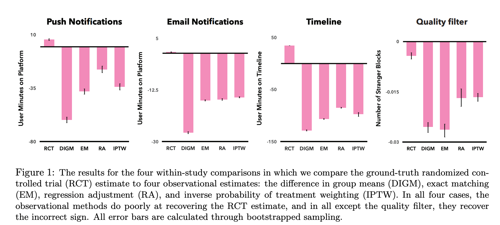
The paper presents a surprising result: for 3 out of 4 within-study comparisons they find that observational methods fail to recover the RCT estimate (even finding an effect with the opposite sign). This is a big deal — it suggests that one should be very careful trying to do causal inference trying to infer the effects of an opt-in feature.
The paper, however, draws a much stronger conclusion, they say: “Our empirical results suggest that observational studies derived from user self-selection are a poor alternative to randomized experimentation on online platforms.”
This blog post is divided into two parts. In the first, I argue that the paper has a methodological issue that can explain the weird result they observe. In the second, I discuss my take on the paper’s top-level message: the apparent tension between causal inference and agency.
Part 1: A methodological issue with the paper
The papers’ methodology is inspired in another paper (Gordon et al. 2019), and goes as follows:
- They divide a small number of randomly sampled users between treatment and control.
- Treatment users can comply with the treatment or not (opt-out).
- Control users never see the treatment
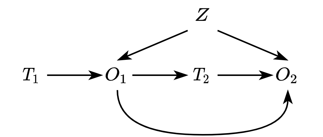
The catch here is that compliance is perfect in the control group, but one-sided in the treatment group. The fact that users can opt-out divides them into “treatment-unexposed” (those that opted-out) and “treatment-exposed” (those that did not). Exposure, therefore, is an endogenous outcome: a user characteristic ($Z$) (e.g., time spent on the platform) can influence both the treatment ($T$) and the outcome ($O$) — in DAG-speak:

In the experimental setting, they estimate the average treatment effect on the treated (ATT), comparing the treatment exposed group, and the control group. In the observational setting, they estimate the ATT comparing the “treatment-exposed” group and the control group. They control for general attributes of the account in the observational setting. Also, it is worth noticing here that the outcome is time spent on Twitter!
Okay, so what’s the problem?
In short, the problem with this method is that the “opting-out” is tied to time spent, therefore, it is almost like we had a third (impossible arrow) in the DAG presented before: the longer you are active, it is more likely that you’ll opt-out of any given feature. In (incorrect) DAG-speak:

We can fix this DAG by decomposing each untreated unit in the observational setting into different periods. For simplicity, let’s assume only 2. The first starts when users are assigned treatment by researchers. Here, treatment ($T_1$) will influence user activity in the first period ($O_1$) but also the status of treatment in the subsequent period! More active users will likely have a higher chance of dropping out! In DAG-speak:
In that context, I don’t think the observational setting here is really valid! In the paper, they always find that the effect is lower for the observational setting, i.e., they reduce their time spent more (see figure below).
The reason why this happens is that users that dropped out likely spent more time on the platform (as they had to log in, drop out, etc). Thus, “treatment-exposed” and “control” are not really comparable! In the discussion of the paper authors state:
A simple fix
How to fix this? It is simple! Get the users that did drop out and decompose their activity in two periods (A and B). This can be done as in the following figure:
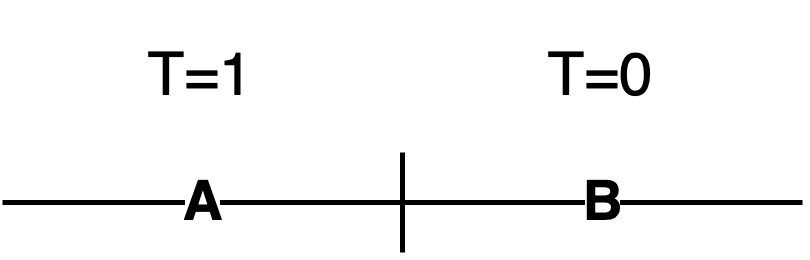
Now you have to get users in the treatment group (who never dropped out) and then try to find matches where they had a period A of similar type with similar activity. In other words, you are matching on the outcome before users in the control group opt-out. This should fix the DAG shown above and allow for a much better estimate of the causal effect.
Part 2: Causal inference and rationality, is there really a problem?
Along with this analysis, the paper also touches upon a more philosophical question: what does it mean to do causal inference when we give users control. Essentially, authors point that there is an apparent contradiction:
- On the one hand, if you are giving users a choice, it means that you are not able to accurately predict what is best for users. Thus, you cannot guarantee the correctness of causal inference.
- On the other hand, if you are doing causal inference, it means that you have a good model of how users behave. If that is the case, and if we can model users so well, it does not make sense to provide them with user controls in the first place.
This view conflates causal inference with “predicting user actions.” For instance, they state:
(…) a major motivation for giving users greater agency is the belief that there is no adequate model for predicting user behavior, however, performing observational causal inference successfully requires exactly that.
Okay, so what’s the problem?
This is not true! You can have a bad model for predicting user behavior (e.g., self-selection into treatment) and still get a good causal estimate.
Instead of justifying this with words, I show it in a minimal example. For instance, consider the first DAG we talked about:
Let’s assume that:
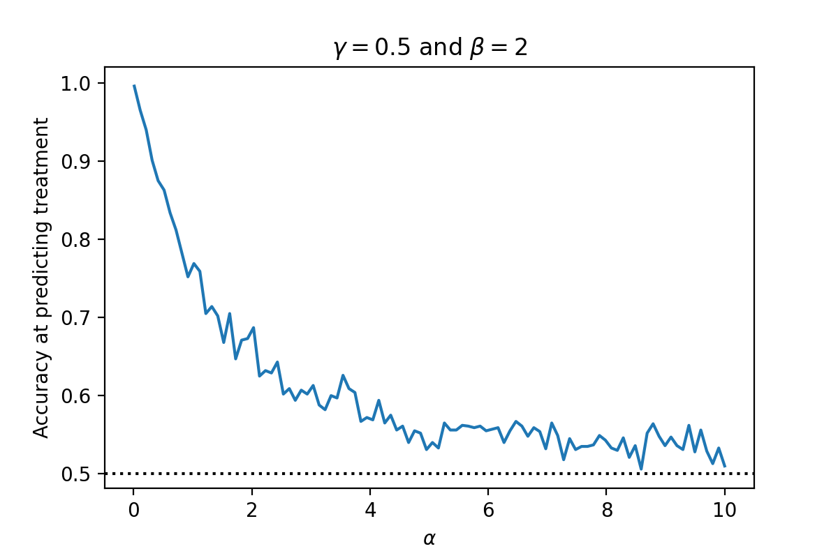
\[\begin{split} Z &\sim N(0, 1) \\ T &= \begin{cases} 1 \qquad \text{if} \quad Z + N(0, \alpha) \geq 0 \\ 0 \qquad \text{otherwise} \\ \end{cases} \\ O &= N(0, \beta) Z + \gamma T \end{split}\]Here, $\alpha$ determines the variance of our treatment given the confounder, $\beta$ determines the variance of our outcome, and $\gamma$ determines the causal effect of the treatment.
If we fix $\gamma = 0.5$ and $\beta = 2$ and vary $\alpha$, we become increasingly worse at predicting treatment. For instance, if we generate samples using the above generative model, varying $\alpha \in [0.01, 10]$, we get the following accuracy at predicting the treatment given $Z$ (using a logistic regression $T = logit(\mu_0 + \mu_1 Z)$):
However, this has absolute no impact on our retrieval of the causal effect. If we estimate the causal effect of $T \to O$ using a simple linear regression $O_i = \mu_0\mu_1 Z_i + \mu_2 T_i$ varying $\alpha \in [0.01, 10]$ we get:
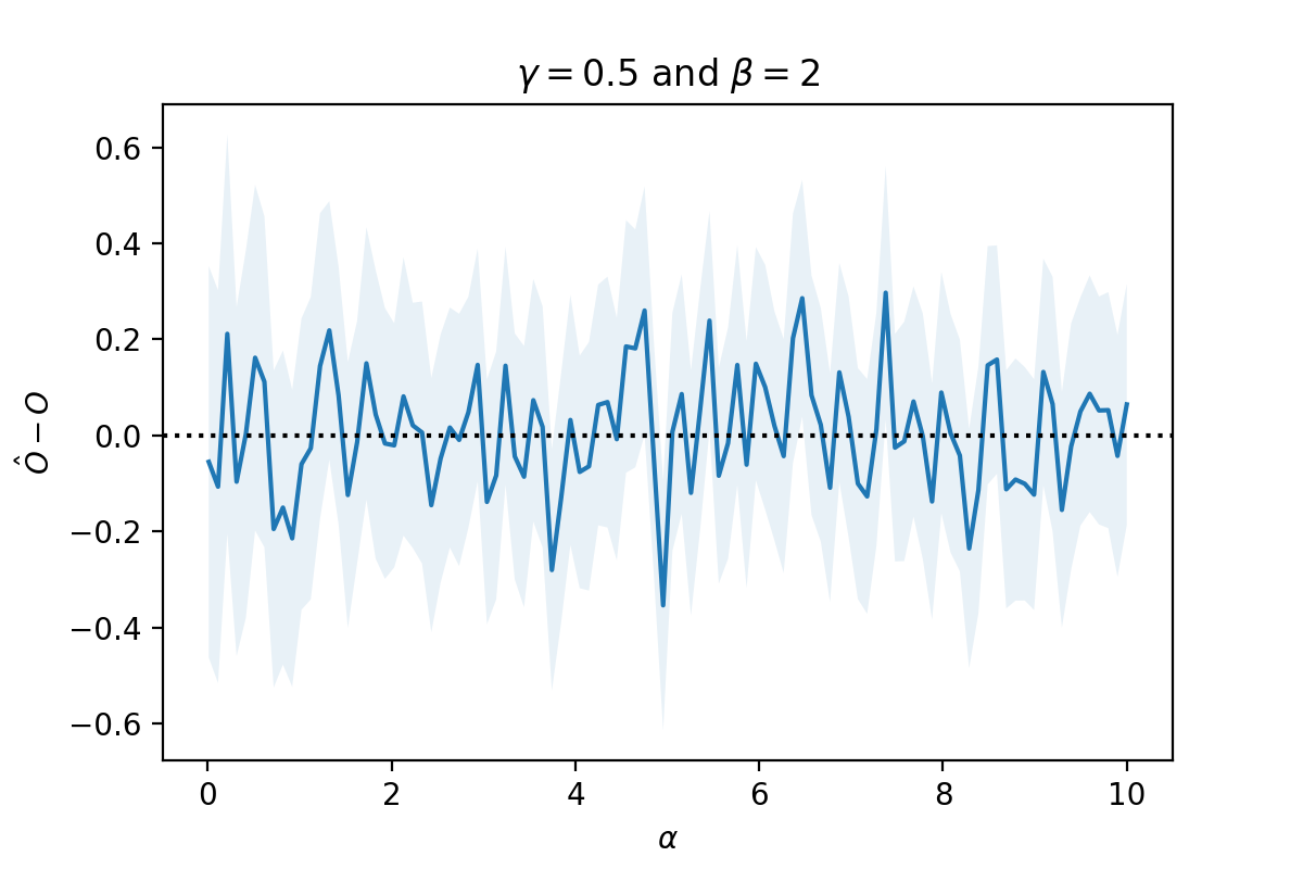
This example disproves the authors’ argument — we have a terrible model to predict a user’s behavior (slightly better than a random guess). However, we can still retrieve the causal effect nicely! You can play with the code used to do these plots in this Google Colab.