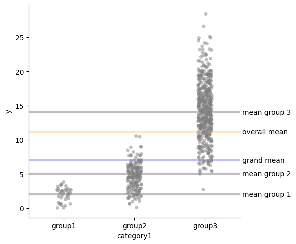
Suppose we are recording a continuous value $y$ for three groups, $group_1$, $group_2$, and $group_3$.
import numpy as np
import pandas as pd
import statsmodels.formula.api as smf
import seaborn as sns
import matplotlib.pyplot as plt
import scipy.stats as stats

group1 = stats.norm.rvs(loc=2, scale=1, size=40)
group2 = stats.norm.rvs(loc=5, scale=2, size=200)
group3 = stats.norm.rvs(loc=14, scale=4, size=500)

df = pd.DataFrame({
    "y": np.concatenate([group1, group2, group3]),
    "category1": ["group1"] * len(group1) +\
                 ["group2"] * len(group2) +\
                 ["group3"] * len(group3)
 })

def plot_mean_and_grand_mean(text=False):
    sns.catplot(x="category1", y="y", data=df, alpha=0.5, color="gray")
    for i, t  in [(2, "mean group 1"), (5, "mean group 2"),
                  (14, "mean group 3"), (7, "grand mean"), (11.15, "overall mean")]:
        color = "black" if i !=7 else "blue"
        color = color if i != 11.15 else "orange"
        plt.axhline(i, color=color, alpha=0.25, lw=3)
        if text:
            plt.text(2.525, i, t, ha="left", va="center")


plot_mean_and_grand_mean(text=True)
plt.show()
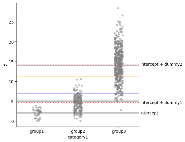
Dummy encoding
We can analyze the groups with a linear model \(Y_i = \alpha_0 + \alpha_1 I_2 + \alpha_1 I_3 + \epsilon_i\) where $I_2$ is an indicator variable for $group_2$ and $I_3$ is an indicator variable for $group_3$. This means that:
- If $i\in group_1$, then $I_2 = 0$ and $I_3 = 0$;
- If $i\in group_2$, then $I_2 = 1$ and $I_3 = 0$;
- If $i\in group_3$, then $I_2 = 0$ and $I_3 = 1$.
We can summarize this using a contrast matrix of shape $levels \times levels - 1$ (here we have 3 levels), so:
\[\begin{matrix} & (I_2) & (I_3) \\ (group_1) & 0 & 0 \\ (group_2) & 1 & 0 \\ (group_3) & 0 & 1 \\ \end{matrix}\]With least squares, we obtain that:
- $\mu_{group_1} = \alpha_0$
- $\mu_{group_2} = \alpha_0 + \alpha_1$
- $\mu_{group_3} = \alpha_0 + \alpha_2$
Proof for the univariate regression case (click to expand)
This can be formally shown if we use the formula for the regression coefficients. Let us consider the case where we have only two groups, and thus
$$ Y_i = \alpha_0 + \alpha_1 I_2 + \epsilon_i $$We have closed formulas for the regression coefficients, namely if $p$ is the percentage of units in group 2, then
$$ \alpha_1 = \frac{Cov(I_2, Y_i)}{Var(I_2)} = \frac{p(\mu_{group_2} - \mu)}{p(1-p)} = \mu_{group_2} - \mu_{group_1} $$ $$ \alpha_0 = E[Y_i] - \alpha_1 E[I_2] = \mu - p (\mu_{group_2} - \mu_{group_1}) = \mu_{group_1} $$Proof for the multivariate regression case (click to expand)
For multivariate linear model ($ Y_i = \alpha_0 + \alpha_1 I_2 + \alpha_2 I_3 + \epsilon_i $), things are a bit trickier, we can use Frisch-Waugh-Lovell Therem to show that:
Any predictor’s regression coefficient in a multivariate model is equivalent to the regression coefficient estimated from a bivariate model in which the residualised outcome is regressed on the residualised component of the predictor
— Lovell, Michael C. 1963. “Seasonal Adjustment of Economic Time Series and Multiple Regression Analysis.” Journal of the American Statistical Association 58 (304): 993–1010.
Thus, we first regress $I_2 = \beta_0 + \beta_1 I_3 + \epsilon_i$. We can get the coefficients using the same formulas we used in the univariate case. Let $a$, $b$, and $c$ be the percentage of units in $group_1$, $group_2$, and $group_3$ respectively. We have that
$$ \begin{align*} \beta_1 &= \frac{Cov(I_2, I_3)}{Var(I_3)} \\ &= \frac{-bc}{c(1-c)} \\ &= \frac{-b}{1-c} \\ \\ \beta_0 &= E[ I_2] - \beta_1 E[I_3]\\ &= b - \frac{-b}{1-c} c \\ &= \frac{b - bc}{1-c} + \frac{bc}{1-c} \\ &= \frac{b}{1-c} \end{align*} $$Replacing the coefficients, we have
$$\hat{I}_2 = \overbrace{\frac{b}{1-c}}^{\beta_0} + \overbrace{\frac{-b}{1-c}}^{\beta_1} I_3.$$Then, given the residual of the previous regression $\tilde{I}_2 = I_2 - \hat{I}_2$, we consider the univariate model:
$$ Y_i = \alpha_1 \tilde{I}_2 + \epsilon_i $$The FWL theorem proves that the $\alpha_1$ of that equation is exactly the same as the $\alpha_1$ of $Y_i = \alpha_0 + \alpha_1 I_2 + \alpha_1 I_3 + \epsilon_i$. We can estimate $\alpha_1$ as:
$$ \alpha_1 = \frac{Cov(Y, \tilde{I}_2)}{Var(\tilde{I}_2)} $$We find that
$$ \begin{align*} E(\tilde{I}_2) &= \frac{1}{n} \sum (I_2 + \frac{-b}{1-c} + \frac{b}{1-c} I_3) \\ & = \frac{1}{n} [ n_1 \frac{-b}{1-c} + n_2 \frac{a}{1-c}] \\ & = a \frac{-b}{1-c} + b \frac{a}{1-c} \\ & = 0 \\ \\ Var(\tilde{I}_2) &= \frac{1}{n} \sum (I_2 + \frac{-b}{1-c} + \frac{b}{1-c} \alpha_1 I_3 - 0)^2 \\ & = \frac{1}{n} [ n_1 \frac{-b}{1-c}^2 + n_2 \frac{a}{1-c}^2] \\ & = a \frac{-b}{1-c}^2 + b \frac{a}{1-c}^2 \\ & = 1 \\ \\ Covar(Y , \tilde{I}_2) &= E[Y (\tilde{I}_2 )] - E[Y] \overbrace{E[I_2 - \hat{I}_2}^{0}] \\ &= \mu_2 a \frac{-b}{1-c} + \mu_1 b \frac{a}{1-c} \\ &= \mu_2 - \mu_1 \\ \end{align*} $$Thus $\alpha_1 = \mu_2 - \mu_1$. Which confirms what we said. To calculate the intercept, we do the same for $\alpha_2$, finding that $\alpha_2 = \mu_3 - \mu_1$. Then we can obtain $\alpha_0$ with the following expansion:
$$ \begin{align*} E(Y - \hat{Y}) &= 0\\ \frac{1}{n} \sum_{i} Y_i - \alpha_0 - \alpha_1 \hat{I}_2 - \alpha_2 \hat{I}_3 &= 0 \\ \mu - \alpha_0 + - b \alpha_1 - c \alpha_2 &= 0 \\ \mu - \alpha_0 + - b (\mu_2 - \mu_1) - c (\mu_3 - \mu_1) &= 0 \\ a \mu_1 + b \mu_2 + c \mu_3 - \alpha_0 - b (\mu_2 - \mu_1) - c (\mu_3 - \mu_1) &= 0 \\ a \mu_1 + b \mu_1 + c \mu_1 &= \alpha_0 \\ \alpha_0 &= \mu_1 \\ \end{align*} $$res = smf.ols("y ~ C(category1)", data=df).fit()
plot_mean_and_grand_mean()
for i, t in [(res.params["Intercept"], "intercept"),
(res.params["Intercept"] + res.params["C(category1)[T.group2]"], "intercept + dummy1"),
(res.params["Intercept"] + res.params["C(category1)[T.group3]"], "intercept + dummy2"),
]:
plt.axhline(i, color="red", alpha=0.75, ls=":")
plt.text(2.525, i, t, ha="left", va="center")
plt.show()
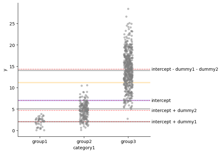
Sum encoding
Alternatively, with the same linear model \(Y_i = \alpha_0 + \alpha_1 I_2 + \alpha_1 I_3 + \epsilon_i\)
we can use a different encoding:
- If $i\in group_1$, then $I_2 = 1$ and $I_3 = 0$;
- If $i\in group_2$, then $I_2 = 0$ and $I_3 = 1$;
- If $i\in group_3$, then $I_2 = -1$ and $I_3 = -1$.
We can summarize this using a contrast matrix:
\[\begin{matrix} & (I_2) & (I_3) \\ (group_1) & 1 & 0 \\ (group_2) & 0 & 1 \\ (group_3) & -1 & -1 \\ \end{matrix}\]With least squares, we obtain that:
- $\alpha_0 = (\mu_{group_1} + \mu_{group_2} + \mu_{group_3}) /3$
- $\mu_{group_1} = \alpha_0 + \alpha_1$
- $\mu_{group_2} = \alpha_0 + \alpha_2$
- $\mu_{group_3} = \alpha_0 - \alpha_1 - \alpha_2$
Proof for the univariate regression case (click to expand)
Let us consider the case where we have only two groups, and thus
$$ Y_i = \alpha_0 + \alpha_1 I_2 + \epsilon_i $$And where if $i\in group_1$ then $I_2 = 1$ and if $i\in group_2$ then $I_2 = -1$.
We have closed formulas for the regression coefficients, namely if $p$ is the percentage of units in group 2, then
$$ \alpha_1 = \frac{Cov(I_2, Y_i)}{Var(I_2)} = \frac{p\mu_1 - q\mu_2 - \mu(p - q)}{4qp} = \mu_1 - \frac{\mu_1 + \mu_2}{2} $$ $$ \alpha_0 = E[Y_i] - \alpha_1 E[I_2] = p \mu_1 + q\mu_2 - (\mu_1 - \frac{\mu_1 + \mu_2}{2}) (p-q) = \frac{\mu_1 + \mu_2}{2} $$res = smf.ols("y ~ C(category1, Sum)", data=df).fit()
plot_mean_and_grand_mean()
for i, t in [(res.params["Intercept"], "intercept"),
(res.params["Intercept"] + res.params["C(category1, Sum)[S.group1]"], "intercept + dummy1"),
(res.params["Intercept"] + res.params["C(category1, Sum)[S.group2]"], "intercept + dummy2"),
(res.params["Intercept"] - res.params["C(category1, Sum)[S.group1]"]\
- res.params["C(category1, Sum)[S.group2]"], "intercept - dummy1 - dummy2")
]:
plt.axhline(i, color="red", alpha=0.75, ls=":")
plt.text(2.525, i, t, ha="left", va="center")
plt.show()
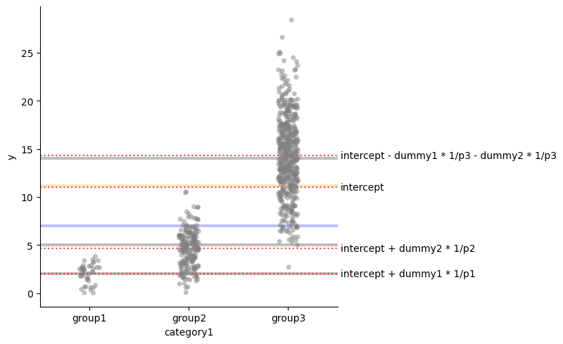
Even cooler encoding!
Last, with the linear model \(Y_i = \alpha_0 + \alpha_1 I_2 + \alpha_1 I_3 + \epsilon_i\)
we can use tweaked version of the sum encoding:
- If $i\in group_1$, then $I_2 = \frac{1}{a}$ and $I_3 = 0$;
- If $i\in group_2$, then $I_2 = 0$ and $I_3 = \frac{1}{b}$;
- If $i\in group_3$, then $I_2 = -\frac{1}{c}$ and $I_3 = -\frac{1}{c}$.
Where $a$, $b$ and $c$, are the proportion of the groups in the data. We can summarize this using a contrast matrix:
\[\begin{matrix} & (I_2) & (I_3) \\ (group_1) & \frac{1}{a} & 0 \\ (group_2) & 0 & \frac{1}{b} \\ (group_3) & -\frac{1}{c} & -\frac{1}{c} \\ \end{matrix}\]With least squares, we obtain that:
- $\alpha_0 = \mu$
- $\mu_{group_1} = \alpha_0 + \frac{1}{a} \alpha_1$
- $\mu_{group_2} = \alpha_0 + \frac{1}{b} \alpha_2$
- $\mu_{group_3} = \alpha_0 - \frac{1}{c} \alpha_1 - \frac{1}{c} \alpha_2$
Proof for the univariate regression case (click to expand)
Let us consider the case where we have only two groups, and thus
$$ Y_i = \alpha_0 + \alpha_1 I_2 + \epsilon_i $$And where if $i\in group_1$ then $I_2 = 1/p$ and if $i\in group_2$ then $I_2 = -1/q$.
We have closed formulas for the regression coefficients, namely if $p$ is the percentage of units in group 2, then
$$ \alpha_1 = \frac{Cov(I_2, Y_i)}{Var(I_2)} = \mu_1 - \mu_2 $$ $$ \alpha_0 = E[Y_i] - \alpha_1 E[I_2] = \mu $$df["dummy1"] = 0
pg1m1 = len(df)/(df["category1"] == "group1").sum()
pg2m1 = len(df)/(df["category1"] == "group2").sum()
pg3m1 = len(df)/(df["category1"] == "group3").sum()
df.loc[df["category1"] == "group1", "dummy1"] = pg1m1
df.loc[df["category1"] == "group3", "dummy1"] = - pg3m1
df["dummy2"] = 0
df.loc[df["category1"] == "group2", "dummy2"] = pg2m1
df.loc[df["category1"] == "group3", "dummy2"] = - pg3m1
res = smf.ols("y ~ dummy1 + dummy2", data=df).fit()
plot_mean_and_grand_mean()
for i, t in [(res.params["Intercept"], "intercept"),
(res.params["Intercept"] + res.params["dummy1"] * pg1m1,
"intercept + dummy1 * 1/p1"),
(res.params["Intercept"] + res.params["dummy2"] * pg2m1,
"intercept + dummy2 * 1/p2"),
(res.params["Intercept"] - res.params["dummy1"] * pg3m1 - res.params["dummy2"]* pg3m1,
"intercept - dummy1 * 1/p3 - dummy2 * 1/p3")
]:
plt.axhline(i, color="red", alpha=0.75, ls=":")
plt.text(2.525, i, t, ha="left", va="center")
plt.show()